Overview
White etching cracks (WECs) are a form of subsurface-initiated rolling contact fatigue failure in hardened bearing steels. They are most commonly observed in rolling element bearings operating near motors or generators, particularly in wind turbine drivetrains.
In WEC failures, cracks typically initiate below the surface, often at a non-metallic inclusion and grow until they reach the raceway surface, forming pits or spalls. Unlike classical bearing fatigue, WEC failures often occur well within the intended design life of the bearing.
The definitive root cause of WEC formation remains unresolved. Current understanding suggests that WECs arise from a combination of mechanical loading, tribochemical reactions, and electrical effects. They are identified metallographically using serial sectioning techniques, where characteristic white etching areas (WEAs) become visible beneath the surface.
What Are White Etching Cracks?
White etching cracks consist of a network of subsurface cracks surrounded by regions of altered microstructure known as white etching areas (WEAs). These crack networks are typically associated with subsurface features such as non-metallic inclusions.
A typical WEC network contains:
- A dominant crack running roughly parallel to the raceway surface
- Numerous secondary cracks branching in multiple directions
- Localised WEAs surrounding portions of the crack network
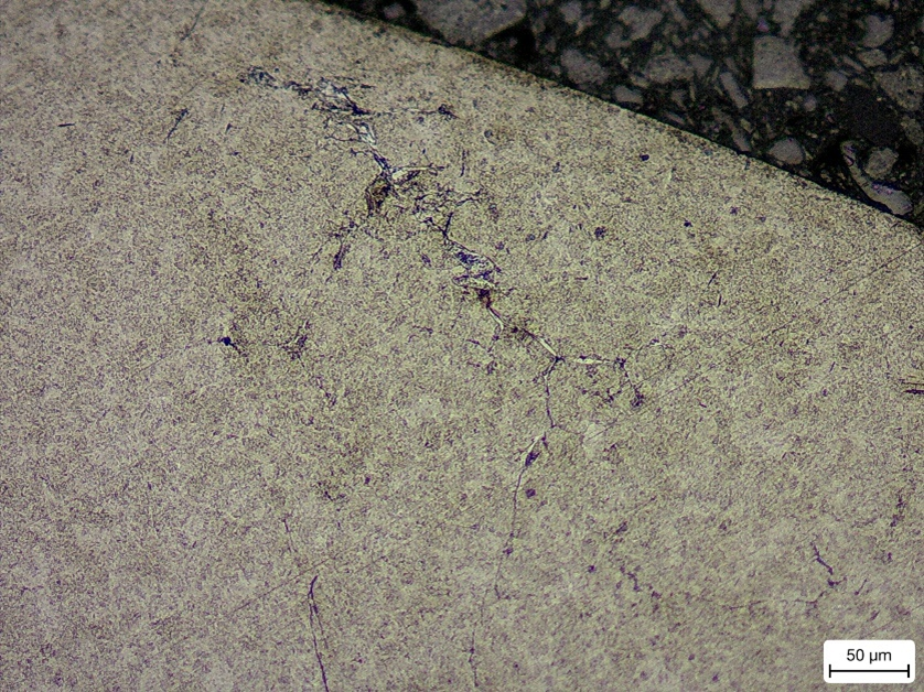
The white etching area is composed primarily of hard ferrite. After polishing and chemical etching, the surrounding martensitic steel etches dark, while the ferritic WEA remains bright, producing a distinctive white appearance under optical or electron microscopy.
In components affected by WECs, many such crack networks are usually present, rather than a single isolated defect.
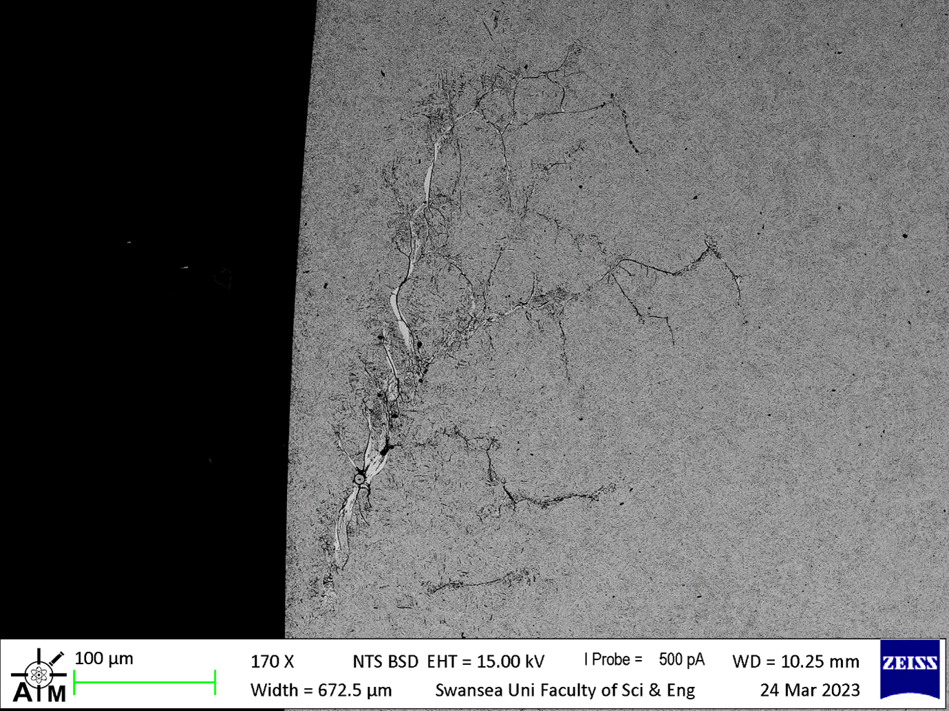
An example SEM image (taken at AIM, Swansea University) illustrates the characteristic features of WEC damage. A small non-metallic inclusion appears to act as the initiation site, with two early-stage “butterfly wings” forming around it. From this region, cracks propagate both parallel to the surface and deeper into the material. Portions of the crack network are bordered by WEAs, indicating significant local microstructural transformation. With continued rolling contact, these subsurface cracks eventually coalesce with the surface, producing a spall or pit.
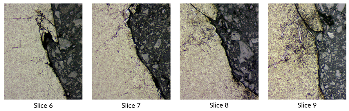
Serial sectioning of a pitted roller (shown below) shows that these crack networks extend through the subsurface. Each section—taken approximately 100 µm apart—reveals a different cross-section of the same interconnected damage structure.
How Is This Different From Classical Pitting
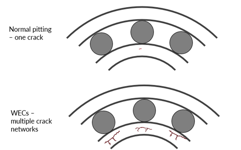
At first glance, WEC failures may appear similar to classical subsurface-initiated pitting, a mechanism that has been well understood for decades. The key differences between the two mechanisms is how the cracks form, how many initiation sites exist, and how the bearing fails statistically.
Classical Subsurface Initiated Pitting
- Typically one initiation site
- One dominant crack leading to one initial pit
- Subsequent damage may occur as debris circulates
- Follows a wear-out failure distribution
- The majority of bearings (>90%) survive beyond their calculated design life
White Etching Crack Failures
- Multiple initiation sites distributed throughout the component
- Many crack networks develop simultaneously
- Cracks are surround by white etching area
- Leads to multiple axial cracks and surface pits
- Failure statistics show early mortality
- Indicates an accelerated damage mechanism, rather than normal fatigue
In WEC-affected bearings, crack networks are often found around the entire circumference of the rolling element or raceway. This indicates that the steel itself has been compromised, making the formation of multiple surface spalls essentially inevitable.
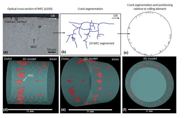
Work by Richardson (1) shown below clearly demonstrates the abundance of crack networks below a steel surface. This was achieved by mapping the location of all crack networks in a single roller specimen, showing widespread subsurface damage long before catastrophic surface failure occurred.
What Causes White Etching Cracks?
In field applications – most notably wind turbines – WEC formation is believed to be driven by a combination of mechanical, electrical, and chemical influences.
Mechanical Drivers
- Transient overloads causing short-duration high contact pressures
(e.g. grid disconnections, emergency stops, wind gusts) - High slip or sliding within the bearing during transient operation
- Edge loading due to misalignment or deflection
Electrical Drivers
- Electrical discharge events
High current or voltage events can create surface damage that locally increases subsurface stress - Stray currents
Lower-level currents can disrupt tribofilm formation, accelerate lubricant degradation, and promote hydrogen generation
Chemical Drivers
- Water contamination, which can act as a source of hydrogen
- Lubricant formulation
Some additive chemistries are associated with increased WEC susceptibility
Oils that form robust, low-friction tribofilms tend to reduce WEC risk - Lubricant oxidation, which may generate hydrogen as a by-product
Competing Theories of WEC Formation
It is increasingly accepted that WEC formation may be multi-modal, with different mechanisms dominating under different operating conditions. The most popular theories include hydrogen embrittlement, transient overloads and electrical current effects.
Hydrogen Embrittlement
Hydrogen diffuses into the steel, reducing ductility and promoting crack initiation and branching. Hydrogen may originate from water contamination or lubricant degradation.
Stress History and Transient Overloads
The transient nature of the wind turbine mechanical system may cause short-duration, high-stress events. These will result in very high pressures or increased sliding in the bearing and may initiate subsurface cracks. These cracks then propagate slowly under normal loading. One hypothesis suggests that rubbing of crack faces contributes to the formation of the white etching area.
Electrical Current Effects
WECs have been generated experimentally under moderate direct and alternating currents (≈250 mA).
The electrical current is known to effect tribofilm formation, possibly hindering it, promoting metal-on-metal contact, which could then lead to higher friction and higher stresses in the subsurface. The lack of a robust tribofilm may also lead to the accelerated oxidation of the lubricant, forming hydrogen.
Current Mitigations in the Field
Lubrication-Based Approaches
- Additive chemistries less prone to hydrogen generation
- Improved oxidative stability
- Controlled lubricant conductivity and polarity
- Reduced water content (typically <200–300 ppm)
- Adequate film thickness and correct viscosity
- Avoidance of overheating
Materials and Surface Engineering
- Ultra-clean steels (fewer inclusions)
- Optimised heat treatments
- Protective coatings (e.g. black oxide, DLC, ceramic coatings)
What Can the Lubricant Do?
The lubricant plays a central role in mitigating WEC formation. Beyond reducing friction and wear, it must form a robust tribofilm capable of maintaining low friction under:
- High loads
- Sliding conditions
- Variable electrical environments
Effective tribofilms help control subsurface stress fields and reduce metal-to-metal contact. This not only limits crack initiation and propagation but may also suppress lubricant degradation pathways that lead to hydrogen generation.
Weibull Statistics and WEC Failures
Weibull statistics are commonly used to describe fatigue failures in rolling contact systems.
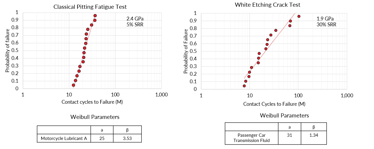
In classical pitting tests, the distribution of cycles to failure is relatively narrow, with a Weibull slope β ≈ 3, characteristic of wear-out behaviour.
In contrast, WEC-type tests exhibit a much lower Weibull slope (β ≈ 1). This indicates early failures, with some specimens failing very quickly while others survive much longer. This statistical signature reinforces the view that WECs represent an accelerated failure mechanism, rather than normal rolling contact fatigue.
The test results shown below use a 3 ring on roller test machine with multiple repeat tests. The classical pitting fatigue test results are taken from the data by Smeeth (2) which uses a SRR of 5% and 2.4 GPa, with 10W-40 motorcycle oils. The white etching crack tests use a SRR of 30 % and 1.9 GPa, and a 75W80 transmission oil.
Laboratory Testing of White Etching Cracks
WECs can be reproduced at laboratory scale using specialised test methods, typically with deliberate acceleration strategies:
- High slide-roll ratios
(e.g. ~30% SRR on MPR or high-slip configurations in FE8 tests) - Hydrogen charging of steels
- Use of known “bad reference oils” (3)
- Lower cleanliness steels with higher inclusion content
- High contact pressures applied early in the test (4)
These approaches allow WEC behaviour to be studied within practical test durations, albeit under deliberately severe conditions. If you would like to learn more about WEC and how we are helping people solve them, please get in touch.
References
- Richardson, A.D., Evans, MH., Wang, L. et al. The Evolution of White Etching Cracks (WECs) in Rolling Contact Fatigue-Tested 100Cr6 Steel. Tribol Lett 66, 6 (2018). https://doi.org/10.1007/s11249-017-0946-1
- Smeeth, M., “The Rolling Contact Fatigue Behaviour of Motorcycle Lubricants,” SAE Technical Paper 2014-32- 0117, 2014, doi:10.4271/2014-32-0117.
- https://www.stle.org/files/TLTArchives/2019/04_April/Cutting_Edge.aspx
- Francesco, M., The Origin of white etching cracks and their significance to rolling bearing failures,” Int. J. Fatigue., 120, (2019) 107-133. https://doi.org/10.1016/j.ijfatigue.2018.10.023


